Digital Paleoseismic Trench Surveying
Tutorial: Digital Paleoseismic Trenching
In this tutorial I want to show you how I’ve been using Structure-from-Motion (SfM) photogrammetry, iOS laser scanning, and an iPad Pro to create accurately scaled digital trench logs in the field.
Requirements: 2020 or newer iPad Pro or iPhone Pro; Agisoft Metashape software; computer.
This tutorial is broken into several different parts. First I will introduce the problems I aim to solve, then I will show you the field data collection and scanning, then the processing workflow, before I finish with a demonstration of how powerful field logging is directly on a properly rectified trench wall image on the iPad.
First, a brief overview of the methods. Structure-from-Motion has quickly become the go-to choice for making a composite image of a trench wall. Using software like Agisoft Metashape, many photographs can be automatically combined into a composite orthophoto mosaic of a trench wall. We use this same method to also build elevation models from drones.
However, in the case of a trench wall, using just raw photos to produce a model can cause two issues:
1) The resulting image will be in totally arbitrary units so we can’t make accurate measurements from the photo.
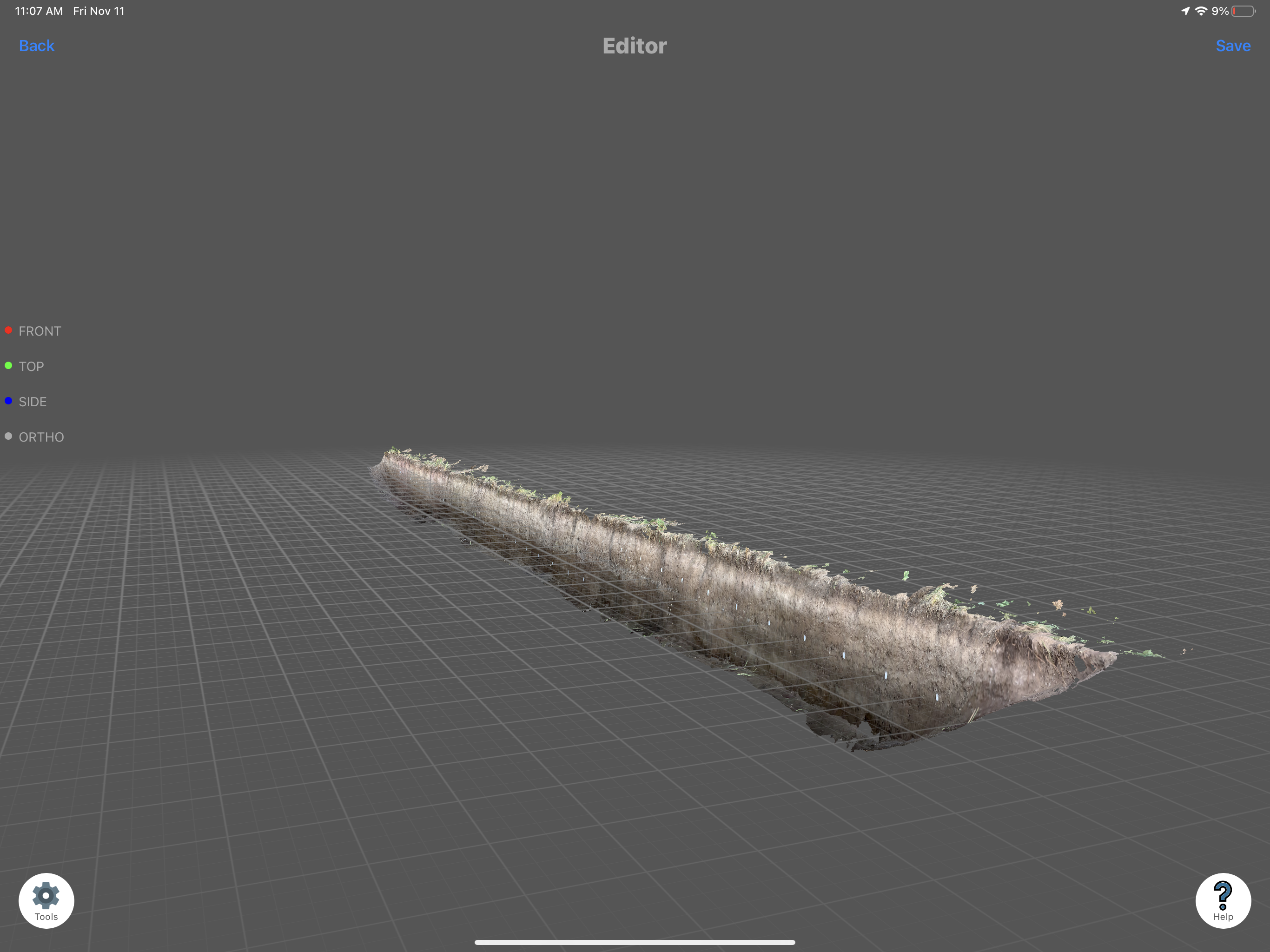
2) Processing the SfM model can produce artifacts such as bowl effects where the trench walls gradually bend and warp towards the camera. This changes the geometry of the trench and prohibits correctly projecting the images to a flat surface.
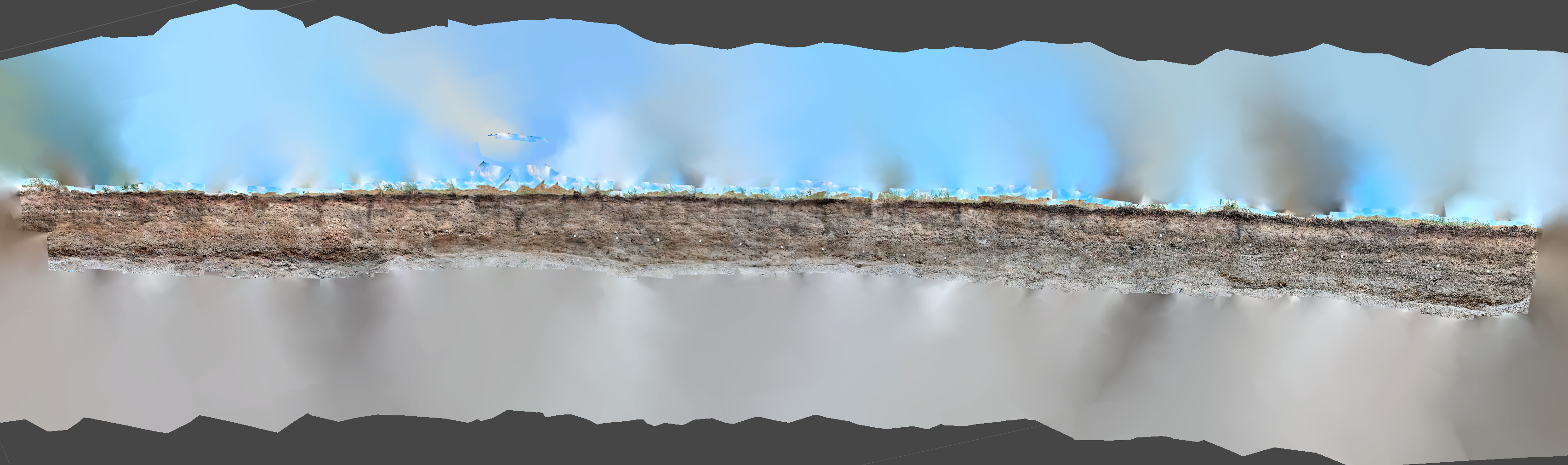
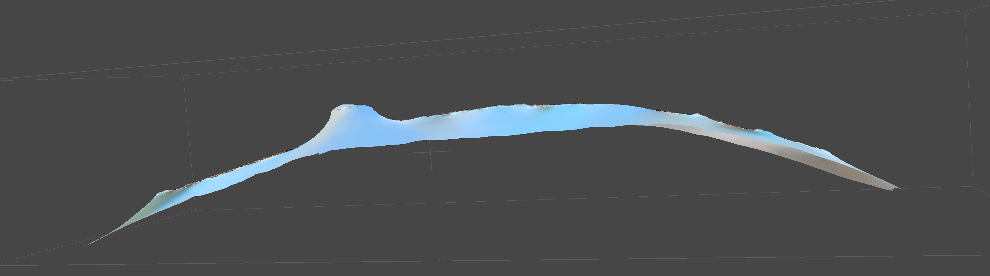
These screengrabs illustrate this example: the model looks OK from the front (upper), but when we look at it from above (lower), we see that what should be a straight trench has a significant curvature.
These issues can be dealt with by either surveying control points throughout the trench exposure, using an expensive total station or differential GPS system (e.g. Reitmann et al., 2015), or by using scale bars, calibrated points that are placed throughout the trench (e.g. Delano et al., 2022). It should be noted that the scale bar method alone is unable to correct for bowl effects.
The method I am describing here is not dissimilar to that using a total station, but instead of requiring this expensive & bulky instrument, I’m using the laser scanner built into the 2020 onward iPhone and iPad Pros to survey the trench and extract control points.
Part 1: Trench Surveying
So now, on to the trench excavation and surveying tutorial. At this point, you’ve dug your trench, cleaned the walls off nicely, and made a grid. I make a grid of nails with clearly labeled flags at 1 m intervals. I use letters to denote the vertical coordinate and numbers for the horizontal coordinate. String grids hanging in front of the wall leave a lot of artifacts in SfM model- so I take the string off before photographing.
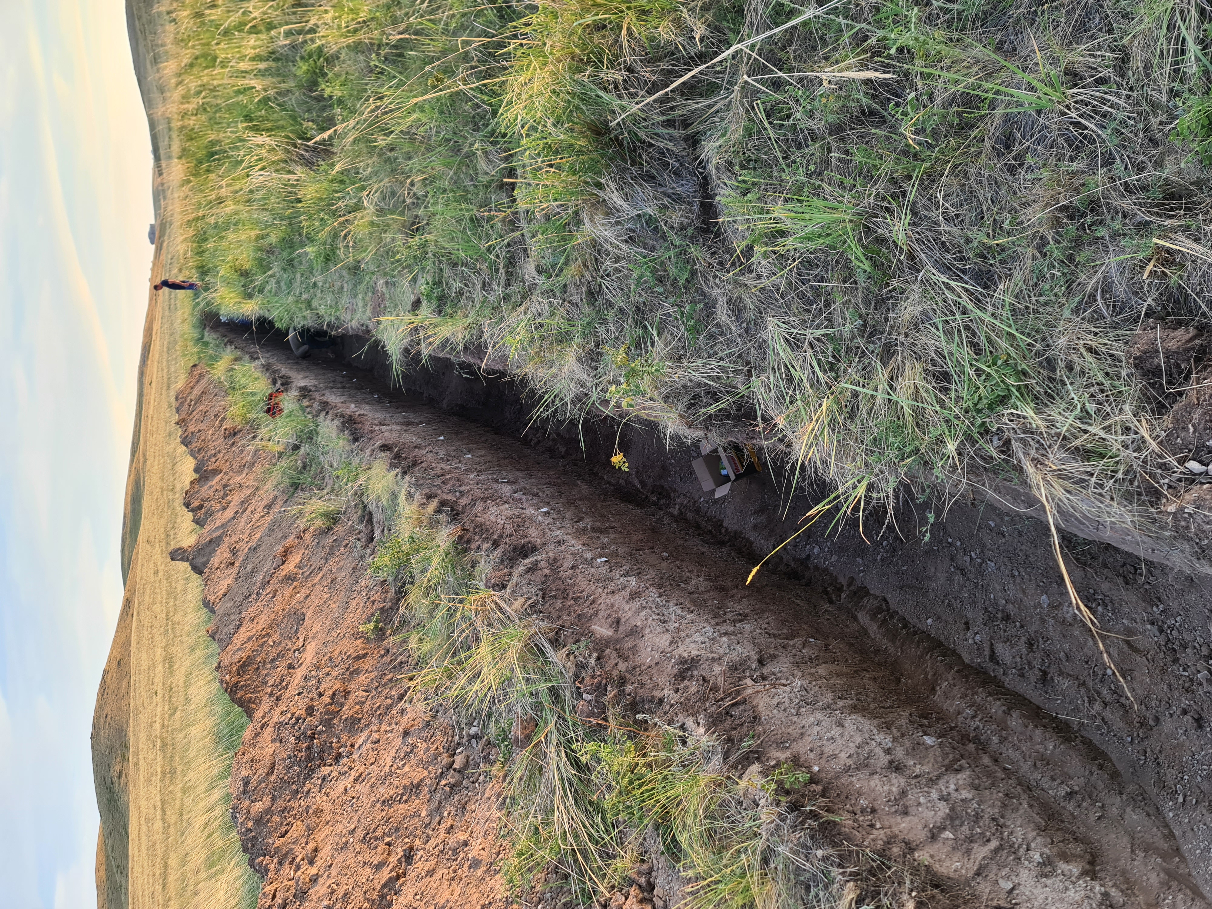
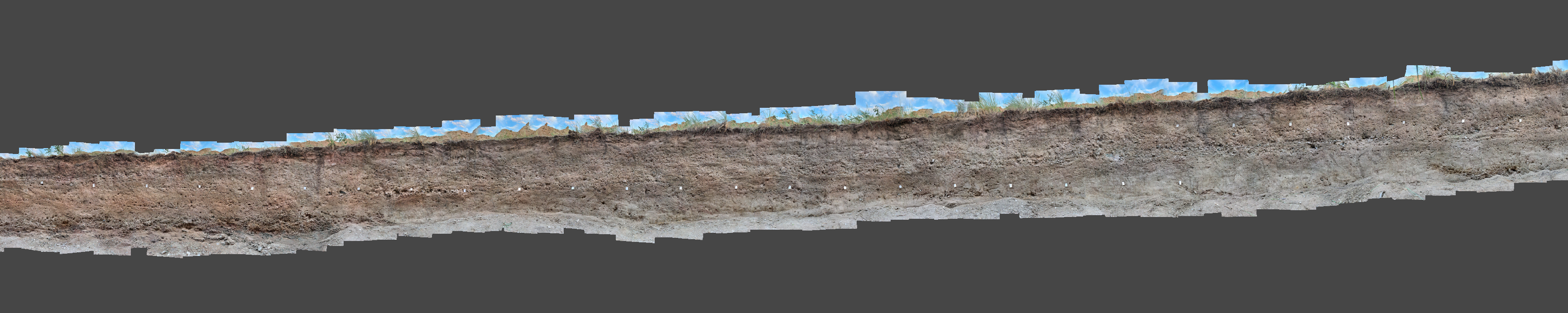
Our beautiful straight trench in the Kazakh steppe.
It doesn’t matter what order you do the next steps in, but next is to take the photos and capture the iOS lidar survey. For both surveys you want to pay attention to the lighting that will be both on the trench wall and on your camera. You want the trench wall to be evenly lit and ideally shaded. In this video you will see we are doing it just after sunset. This ensures there is still enough light but that the wall won’t have shadows and the camera won’t have lens-flare issues.
For the photos I use my cell phone camera. I have a Samsung Galaxy S20 Ultra. I put the phone on a monopod that has an adapter for holding the phone. I am using a cheap Bluetooth shutter trigger to take the pictures. Our trench in this example is very narrow and not too deep, so it is easy enough to stand outside the trench to take the photos. In a bigger trench I would stand inside the trench, and if it was benched I would take another set from on each bench.
This video shows my methodology. Starting at one end of the trench, I lower the camera into the trench and take photos, facing straight at the opposite wall, as far from the opposite wall as possible, and at different levels. In this trench I take photos at 4 different levels. I then take about a half meter step down the trench, and repeat the process. If my first set of 4 photos was taken descending, the adjacent set would be taken in an ascending manner, and then descending and so on. I continue this lawn mower pattern down the whole trench. None of the photos are taken oblique to the trench wall, and I try to keep the camera as orthogonal as possible.
Screengrab showing part of the photo capture pattern.
For the 36 m long and 1.7 m deep trench in this example, I took 272 photos. I recommend immediately transferring these photos to a laptop and building a model using low settings. This ensures that your photos will correctly align and build a model. Even after having made models of trench walls dozens of times, I still occasionally will get a set of photos that won’t align for some unknown reason, and you don’t want to waste time waiting for perfect lighting again because your photos didn’t align.
Now for the iOS laser scanning. There are several apps you can use, and I have had good results with 3D Scanner App and Polycam. Here I am using the 3D Scanner App. This is quite simple as it is captured in real time. I slowly walk along the exposure while it is recording. If it was a bigger exposure I would be slowly rotating the iPad to capture all of it. When I get to the other end I tell it to stop recording and then process it using the highest settings. This screengrab shows the resulting scan, processed within a few minutes after capture. I can make measurements directly in this app, and can see that the geometry is quite close to what we see in the field. Note the lack of any bowl effects. I recommend to clean up the model a bit in the app, cropping out areas that are unnecessary.
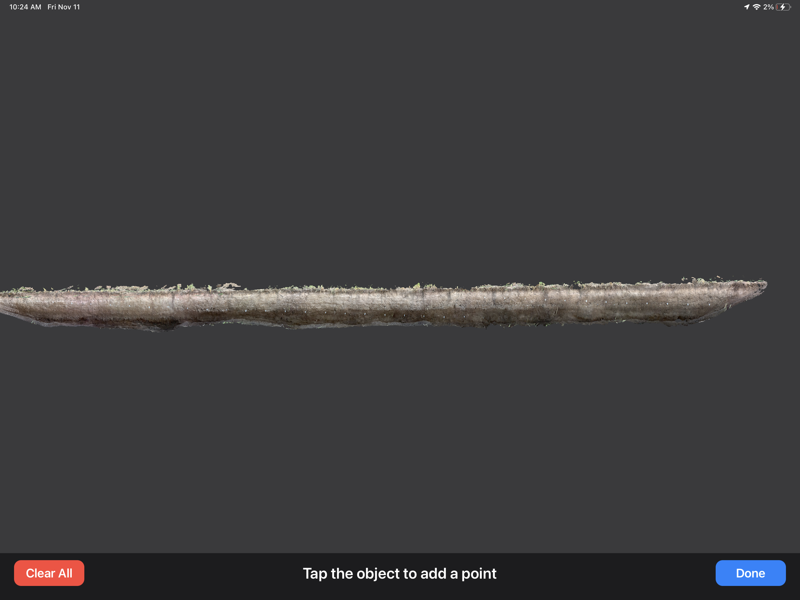
iPad screengrab from 3D Scanner App, note how straight the trench is and the lack of bowl effects.
That’s it. For trenches like this, if I have the laptop set up in the truck, capturing both photos and the lidar scan, and doing a quick, low-settings SfM process takes me about 20 minutes.
Part 2: Data Processing
Now for the trick: how to combine these two scans to add a spatial reference and fix the nasty bowl effects.
First, on the iOS device, export the lidar scan as a .OBJ file and transfer it to your computer. Then, in Agisoft Metashape, in a new empty chunk, go to File > Import > Import Model, and import the scan using local coordinates. It is important that you do this before importing any photos. Now, look at your model and right click on your grid flags to add markers. Zoom into the model to see the name of the markers, and rename the placed markers following the names you read off the tags (e.g. A1, A2, etc.). You don’t need to place every grid marker, but you should make sure they are evenly distributed throughout the scene.
Agisoft Metashape screengrab showing placing markers on the iOS lidar scan.
Once you’ve placed your markers, save your project. Then go to the Reference tab, open the Settings menu, and set the marker coordinate system to Local Coordinates and the marker accuracy to 0.05 m. Note that here I am assuming that the iOS scan has an accuracy of 5 cm.
Agisoft Metashape screengrab showing all markers placed on the iOS lidar scan.
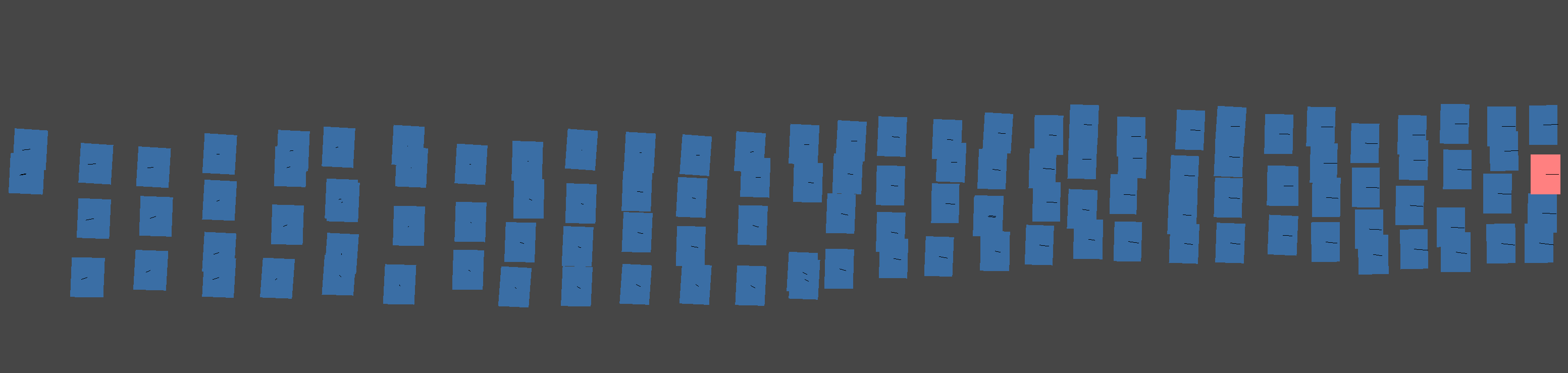
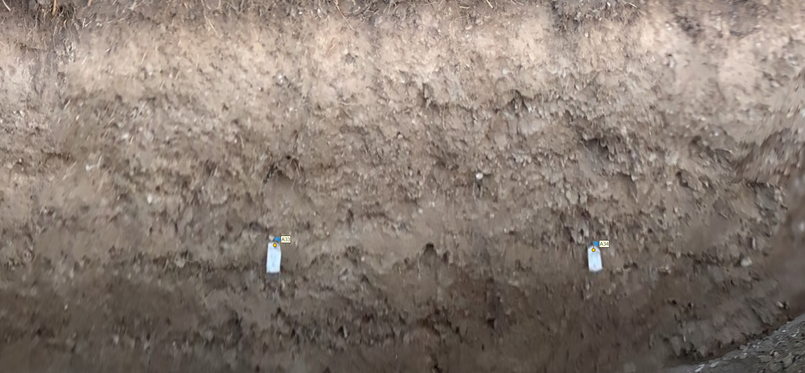
Now import your photos (Workflow > Add Photos, select all photos and import). Then on the pane, go through each photo and place the markers. Right click the marker in the photo, then Place Marker, and select the marker you see. Note that at this stage you don’t actually need to place all the markers you located in the prior step, but it is critical to do a few that are well distributed throughout the trench. The software will estimate the marker locations in the next step and you can then adjust those to save a bit of your time having to manually locate and place them all. In this photo you can see the markers I placed for this project. It is easy to place many more than this if desired.
Metashape screengrab showing marker placement on photos.
Once you’re done putting the markers in the photos, save your project again. Now go to Workflow>Align Photos. I am running this model at High Accuracy, with Generic Preselection and Reference Preselection (Sequential) checked. Under Advanced, Key point limit: 150,000; Tie point limit: 6,000; and adaptive camera model fitting checked. If you haven’t placed all your markers yet, run it at “Low” to save time.
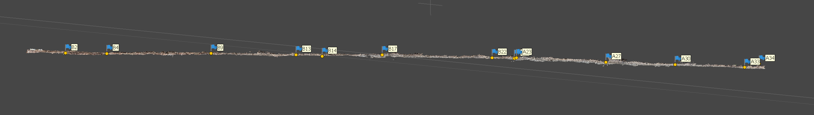
When the alignment finishes, things might look weird. Go to the reference tab, select Optimize Cameras, accept the default settings, and push OK. Then push the update transform. Now you should see your model properly aligned to your markers. Your lidar model might disappear in this process, but you can re-import it the same way as before (File > Import > Import Model). You should see that the sparse cloud and model are pretty well aligned.
Next, if you didn’t place all your markers before, go through and select any photos with gray flags and adjust the markers onto the labels in the photos. Then redo the alignment using high settings.
Run this and go get a cup of coffee while you wait for it to process…
When it finishes, redo the Optimize Cameras step, and select Adaptive camera model fitting. Then clean up your sparse cloud by deleting any extraneous points that are outside of your trench. Inspecting the sparse cloud, we can see it has been successfully de-warped and no longer has the fishbowl effect.
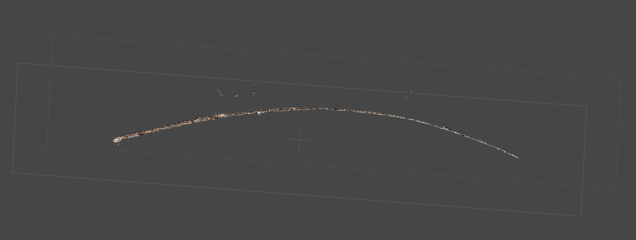
Pre (upper) and post (lower) correction showing the removal of the bowl effect.
Since we are mainly interested in building an orthophoto mosaic, we don’t care about a dense cloud. So we go directly to building the mesh from the sparse cloud. If you were going to continue working in 3D, you might want to build a dense cloud.
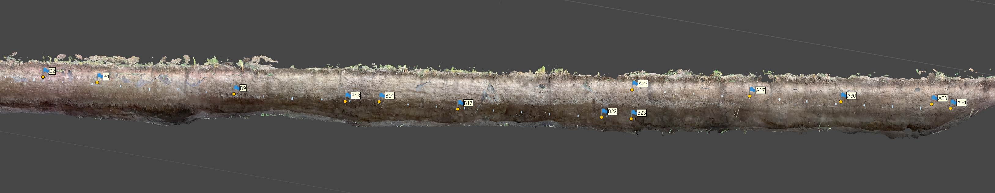
After the mesh has finished, we build the orthophoto mosaic. Workflow > Build Orthomosaic. We can use what we know about our grid to properly project our orthomosaic. On the Build Orthomosaic tab select Planar. Project plane: Markers. Horizontal Axis: choose two markers that are farthest away on a horizontal line, in my case I will use B2 -> B23. Then choose two markers that describe an ascending vertical line, here: B23->A23. Push OK. When that finishes processing, inspect your model.
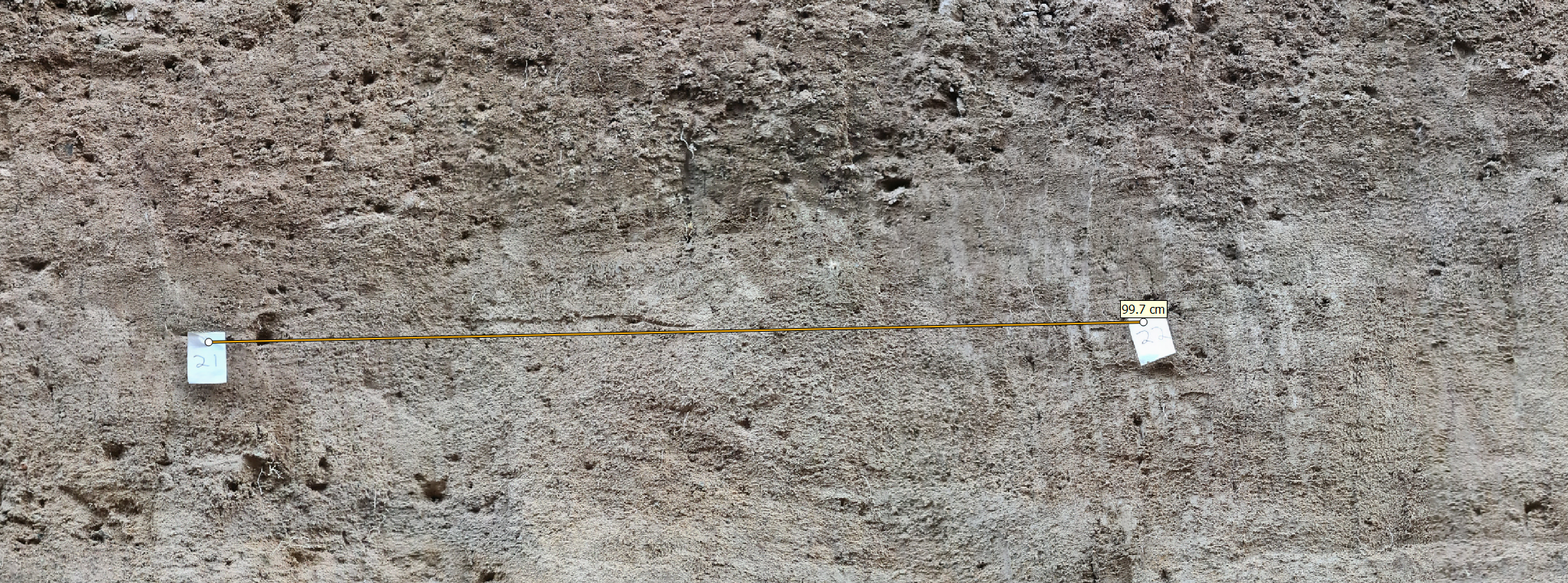
Finished orthomosaic. I can get a rough check on accuracy using the measure tool and measuring between two grid cells. In my case it is pretty good since the 99.7 cm measurement matches the field placement of the 1 m grid. This can be done in a more robust manner if some of the markers are used as check points.
When you are happy with your model, go to export Orthomosaic (File > Export > Export Orthomosaic). Adjust the pixel size so that your final file size is manageable and you have the resolution you want. Under Compression, change TIFF compression to JPEG. Push export and choose a save location and sensible file name.
Congratulations! You’ve finished processing.
Part 3: iPad Field Logging
In the final part of this tutorial I will show you how I log in the field, directly on your orthophoto using an iPad and the Pencil tool.
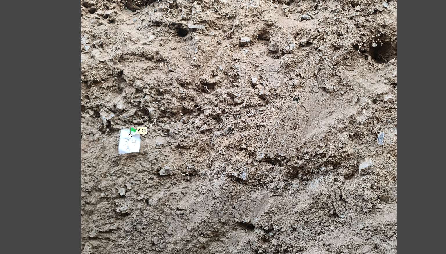
I use Adobe Illustrator, but you can do this with most vector drawing apps. With Illustrator, I open a new document on my computer. I then import my photomosaic and crop away the ugly parts. Then I save it to the cloud. On my iPad I then open the cloud document and can start drawing directly on the orthophoto. I can zoom and pan around the trench with more detail than is typically possible by printing paper photos out. I can turn layers on and off and use the Apple Pencil to draw different lines, polygons, and text notes. This immediately syncs back to the cloud when I go online, and all the annotations are editable on my computer. With other vector apps you will probably have to manually transfer the file back and forth, but the same workflow applies. This saves a ton of time and effort having to hand draw and then scan and reinterpret hand drawings later on. Be warned that these apps are power hungry, so plan to keep a power bank or two strapped to the iPad.
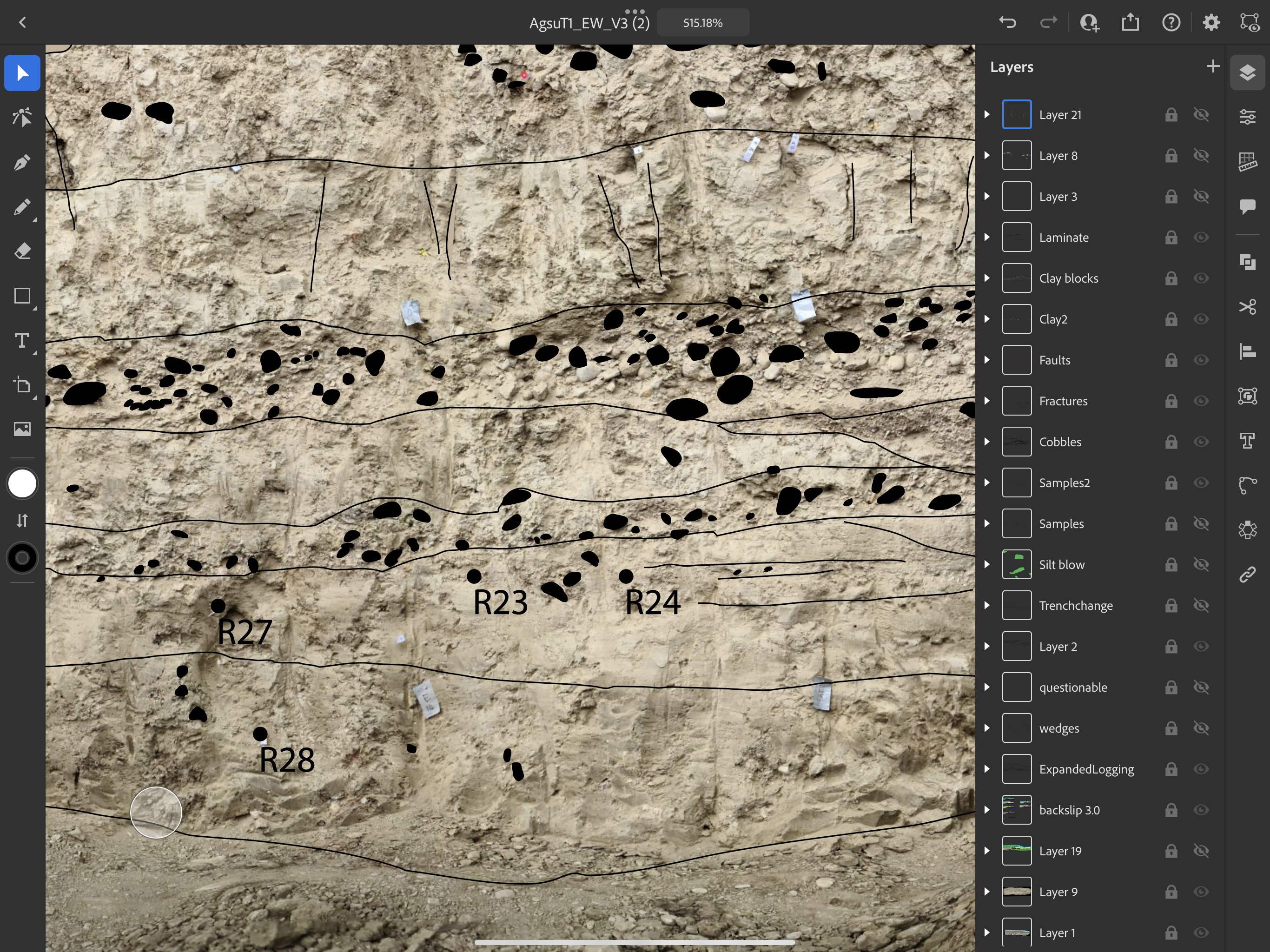
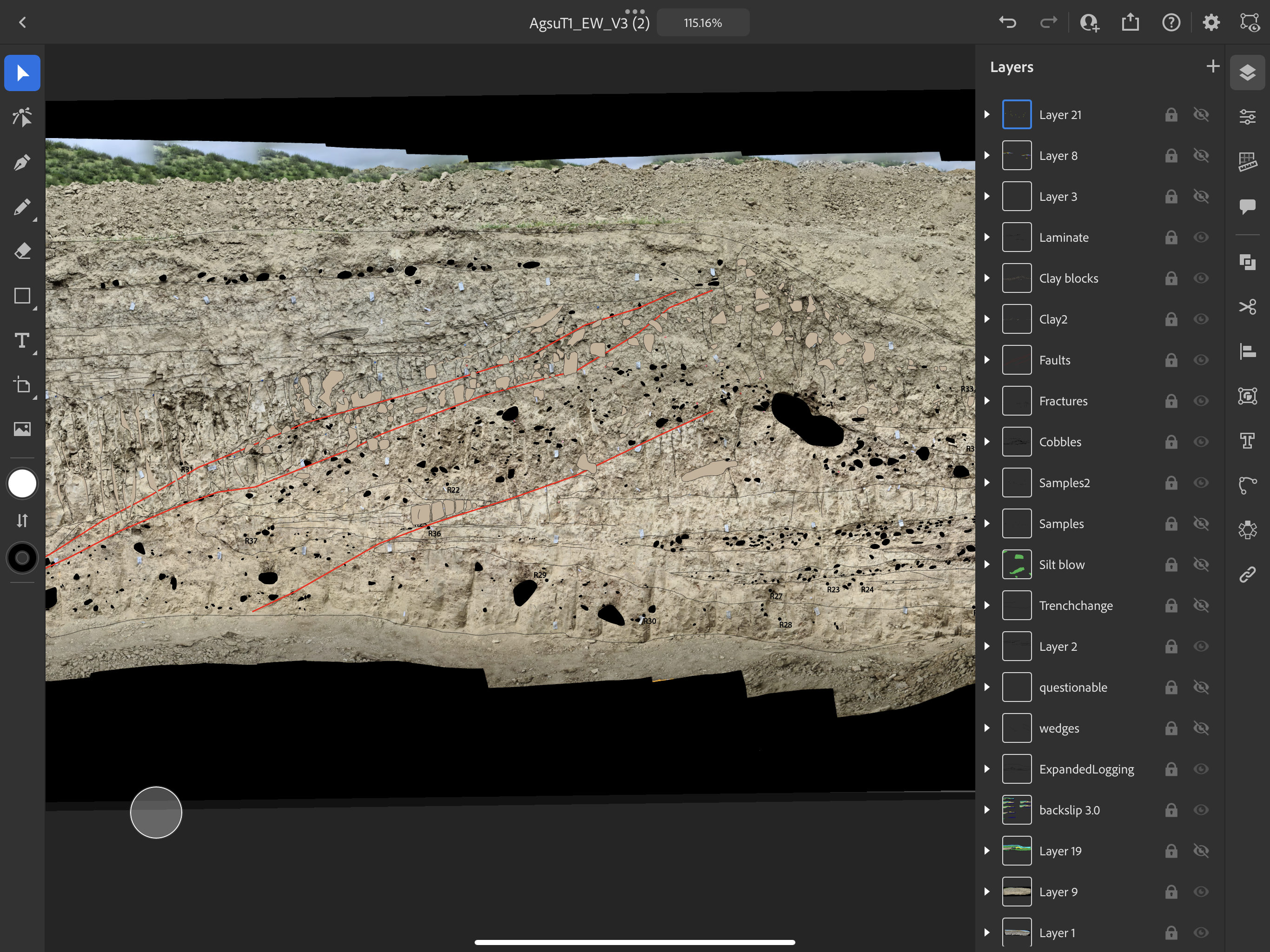
iPad screengrabs showing logging in the Adobe Illustrator iOS app. Note the different layers and full illustrator functionality.
That’s it! If you made it this far I hope you enjoyed the tutorial, and happy trenching!